此文章是依据AI生成的模型案例来制作的通用模版,用于在相似的模型下进行套用,详细的学习笔记见
数学建模建议掌握的模型
五一赛
| 类别 | 算法 | 应用场景 | 工具 |
|---|---|---|---|
| 数据分析与预测 | 线性回归、时间序列分析(ARIMA)、机器学习(随机森林、神经网络) | 能源消耗趋势预测、电力负荷变化预测、复杂多变量预测 | Python (sklearn, statsmodels, TensorFlow, PyTorch), MATLAB |
| 优化 | 线性规划(LP)、遗传算法(GA) | 电力系统调度优化、多参数调节优化 | MATLAB (linprog, ga), Python (PuLP, DEAP) |
| 数值计算 | 数值积分与微分方程 | 电采暖负荷仿真 | MATLAB (ode45), Python (scipy.integrate) |
评价模型
一.层次分析法(AHP)
案例背景
目标:选择最佳旅游地(杭州、桂林、三亚)
准则:景色、费用、居住条件、饮食、交通
1.建立层次结构(需要画图,WPS,draw.io等软件)
- 目标层:最佳旅游地
- 准则层:5个评价准则
- 方案层:3个备选方案
2. 定义函数计算权重和一致性比率(将此函数放辅助函数后,或者放入函数文件中)
function [w, CR, CI] = ahp_weights(A)
% 输入判断矩阵A,返回权重w、一致性比率CR和一致性指标CI
[n, ~] = size(A);
[V, D] = eig(A);                   % 计算特征值和特征向量
[max_eigval, idx] = max(diag(D));  % 最大特征值及索引
w = V(:, idx);                     % 对应特征向量
w = w / sum(w);                    % 归一化权重
CI = (max_eigval - n) / (n - 1);   % 一致性指标
RI = [0 0 0.58 0.90 1.12 1.24 1.32 1.41 1.45 1.49]; % 随机一致性指标表
CR = CI / RI(n);                   % 一致性比率
end功能:计算判断矩阵的权重向量、一致性比率(CR)和一致性指标(CI)。若CR < 0.1,判断矩阵通过一致性检验。
3. 主程序:输入判断矩阵并计算
%% 主程序
% 准则层判断矩阵A(5x5)
A = [1   3    5    4    7;
     1/3 1    3    2    5;
     1/5 1/3 1    1/2  3;
     1/4 1/2 2    1    3;
     1/7 1/5 1/3 1/3 1];

% 计算准则层权重及检验
[w_A, CR_A, CI_A] = ahp_weights(A);
fprintf('准则层权重:\n'); disp(w_A);
fprintf('准则层CR=%.4f,结果:%s\n\n', CR_A, ifelse(CR_A<0.1,'通过','不通过'));

% 方案层判断矩阵B(每个准则对应3x3矩阵)
B = {[1 2 5; 1/2 1 3; 1/5 1/3 1],    % 景色
     [1 1/3 1/5; 3 1 1/2; 5 2 1],    % 费用
     [1 1/3 1/2; 3 1 2; 2 1/2 1],    % 居住
     [1 1 3; 1 1 2; 1/3 1/2 1],      % 饮食
     [1 2 3; 1/2 1 2; 1/3 1/2 1]};   % 交通

% 计算各准则下方案权重及检验
w_B = zeros(3,5); CI_B = zeros(1,5);
for i = 1:5
    [w, CR, CI] = ahp_weights(B{i});
    w_B(:,i) = w;
    CI_B(i) = CI;
    fprintf('准则%d方案权重:\n', i); disp(w);
    fprintf('准则%d CR=%.4f,结果:%s\n\n', i, CR, ifelse(CR<0.1,'通过','不通过'));
end

% 计算总排序得分
total_score = w_B * w_A;
fprintf('各方案总得分:\n'); disp(total_score);

% 总排序一致性检验
CI_total = sum(CI_B .* w_A');        % 总CI
RI_total = 0.58;                    % 方案层RI均为0.58(n=3)
RI_A = 1.12;                        % 准则层RI(n=5)
CR_total = (CI_total + CI_A) / (RI_total + RI_A);
fprintf('总排序CR=%.4f,结果:%s\n', CR_total, ifelse(CR_total<0.1,'通过','不通过'));

% 辅助函数
function s = ifelse(cond, t, f)
    if cond, s = t; else, s = f; end
end使用说明:
- 修改判断矩阵:直接修改代码中的
A和B矩阵数据即可应用于其他AHP问题 - 扩展性:
- 修改准则数量:调整
A矩阵维度 - 修改方案数量:调整
B矩阵维度
- 修改准则数量:调整
- 验证一致性:所有 CR 值自动检查,结果中会明确标注是否通过检验
优化模型
——lingo/lindo软件可行
一.线性规划
案例背景:生产计划优化
目标:某工厂生产两种产品A和B,需合理分配资源以实现最大利润。
数据:
- 每生产1单位A产品需材料2吨,人工3小时,利润300元。
- 每生产1单位B产品需材料4吨,人工1小时,利润200元。
- 每日材料限制为100吨,人工限制为90小时。
1. 定义线性规划模型参数
% 目标函数系数(注意:linprog默认求最小值,因此最大化需取负)
f = [-300; -200];  % 利润系数取负,转为最小化问题

% 不等式约束矩阵(Ax ≤ b)
A = [2, 4;     % 材料约束系数
     3, 1];    % 人工约束系数
b = [100; 90]; % 资源上限

% 等式约束(本问题无等式约束,设为空)
Aeq = [];
beq = [];

% 变量下界(x₁ ≥ 0, x₂ ≥ 0)
lb = [0; 0];解释:
f:目标函数系数向量,由于linprog默认求解最小化问题,需将最大化目标函数系数取负。A和b:不等式约束的系数矩阵和右侧常数项。lb:变量下界,表示生产量不能为负数。
2. 调用linprog求解线性规划
% 调用linprog求解
[x, fval, exitflag] = linprog(f, A, b, Aeq, beq, lb);

% 输出结果
if exitflag == 1
    fprintf('最优解:\n');
    fprintf('生产A产品数量 x₁ = %.2f 单位\n', x(1));
    fprintf('生产B产品数量 x₂ = %.2f 单位\n', x(2));
    fprintf('最大利润 Z = %.2f 元\n', -fval); % 还原为正值
else
    fprintf('未找到可行解或问题无界。\n');
end参数说明:
x:最优解向量(决策变量值)。fval:目标函数最优值(由于目标函数取负,实际利润为-fval)。exitflag:求解状态标识,1表示成功找到最优解。
二.整数线性规划
——经典问题:背包问题,指派问题;
常用算法:蒙特卡洛模拟,动态规划
案例背景:项目投资决策
目标:某公司有500万元预算,需从5个潜在项目中选择若干项目投资,使预期收益最大化。
数据:
| 项目 | 投资(万元) | 预期收益(万元) |
|---|---|---|
| 1 | 150 | 50 |
| 2 | 200 | 80 |
| 3 | 80 | 30 |
| 4 | 120 | 40 |
| 5 | 90 | 25 |
1. 定义整数线性规划模型参数
% 目标函数系数(最大化总收益,需转为最小化问题)
f = -[50; 80; 30; 40; 25];  % 收益取负,转为最小化问题

% 不等式约束(总投资 ≤ 500万元)
A = [150, 200, 80, 120, 90];  % 各项目投资额
b = 500;                       % 总预算上限

% 等式约束(本问题无等式约束)
Aeq = [];
beq = [];

% 变量下界和上界(0-1变量)
lb = zeros(5, 1);    % 下界全为0
ub = ones(5, 1);     % 上界全为1

% 指定整数变量(所有变量为0-1整数)
intcon = 1:5; % 变量x₁到x₅均为整数解释:
f:目标函数系数向量,linprog默认求解最小化问题,因此将收益系数取负。A和b:不等式约束表示总投资不超过500万元。lb和ub:变量范围为0或1(二进制变量)。intcon:指定所有变量为整数(此处为0-1变量)。
2. 调用intlinprog求解整数线性规划
% 调用intlinprog求解
[x, fval, exitflag] = intlinprog(f, intcon, A, b, Aeq, beq, lb, ub);

% 输出结果
if exitflag == 1
    fprintf('===== 最优投资方案 =====\n');
    fprintf('选中的项目:');
    fprintf('项目%d ', find(x > 0.5));
    fprintf('\n总收益: %.2f 万元\n', -fval);  % 还原为正值
    fprintf('总投资: %.2f 万元\n', A*x);
else
    fprintf('未找到可行解。\n');
end参数说明:
intlinprog是MATLAB中用于求解混合整数线性规划的函数。exitflag = 1表示找到可行解。find(x > 0.5)用于定位被选中的项目(因数值解可能接近0或1,需容差处理)
常见问题解答
- 为什么解中出现小数(如x=0.999)?
- 浮点数计算误差导致,可通过
round(x)或x > 0.5处理。
- 浮点数计算误差导致,可通过
- 如何加速求解?
- 减少变量数量、简化约束条件,或设置
Heuristics和CutGeneration选项。
- 减少变量数量、简化约束条件,或设置
- 问题无解怎么办?
- 检查约束是否矛盾(如预算不足以投资任何项目)。
- 放松约束条件或调整目标函数
动态规划
案例背景:0-1背包问题
目标:给定背包容量和一组物品(每个物品有重量和价值),选择物品装入背包,使得总价值最大,且总重量不超过背包容量。
输入:
- 背包容量 W=10W=10
- 物品列表:物品编号重量价值12623834124515
输出:最大总价值及选中的物品编号。
动态规划解决步骤
- 定义状态:
- dp[i][w]dp[i][w]:前 ii 个物品在背包容量为 ww 时的最大价值。
- 目标:求 dp[n][W]dp[n][W],其中 nn 是物品总数。
- 状态转移方程:
- 若物品 ii 重量 >w>w,无法选择:
dp[i][w]=dp[i−1][w]dp[i][w]=dp[i−1][w] - 若物品 ii 重量 ≤w≤w,选择最大价值:
dp[i][w]=max(dp[i−1][w], dp[i−1][w−weight(i)]+value(i))dp[i][w]=max(dp[i−1][w], dp[i−1][w−weight(i)]+value(i))
- 若物品 ii 重量 >w>w,无法选择:
- 初始化:
- dp[0][w]=0dp[0][w]=0(无物品时价值为0)
- dp[i][0]=0dp[i][0]=0(容量为0时价值为0)
- 填表求解:
按物品和容量从小到大填充二维表格。 - 回溯最优解:
从 dp[n][W]dp[n][W] 逆向追踪选择的物品。
% 0-1背包问题动态规划解法(正确版本)
clc; clear;

%% 输入数据
W = 10;
weights = [2, 3, 4, 5];
values = [6, 8, 12, 15];
n = length(weights);

%% 1. 初始化动态规划表
dp = zeros(n+1, W+1);

%% 2. 填充动态规划表
for i = 1:n
    for w = 0:W
        if weights(i) > w
            % 无法选择当前物品
            dp(i+1, w+1) = dp(i, w+1);
        else
            % 注意:w+1 - weights(i) 必须 ≥1
            prev_weight_idx = w + 1 - weights(i);
            if prev_weight_idx < 1
                prev_value = 0;
            else
                prev_value = dp(i, prev_weight_idx);
            end
            dp(i+1, w+1) = max(dp(i, w+1), prev_value + values(i));
        end
    end
end

%% 3. 回溯最优解
selected = [];
remaining_weight = W;
for i = n:-1:1
    current_value = dp(i+1, remaining_weight + 1);
    if current_value ~= dp(i, remaining_weight + 1)
        selected = [selected, i];
        remaining_weight = remaining_weight - weights(i);
    end
end
selected = sort(selected);

%% 4. 输出结果
fprintf('===== 0-1背包问题动态规划解 =====\n');
fprintf('最大总价值: %d\n', dp(n+1, W+1));
fprintf('选中的物品编号: %s\n', num2str(selected));
fprintf('总重量: %d (限额%d)\n', sum(weights(selected)), W);dp表多出一行一列,方便处理边界条件(无物品或容量为0的情况)- 从最后一个物品开始,若当前价值与前一行不同,说明选中了该物品。
- 更新剩余容量,继续向前检查。
动态规划优势:
- 时间复杂度:O(nW)O(nW),伪多项式时间。
- 空间优化:可压缩为一维数组减少空间占用。
- 对比暴力枚举:避免重复计算子问题,显著提升效率。
三.非线性规划问题
——经典问题:
常用算法:蒙特卡洛模拟,局部搜索算法,遗传算法
案例背景:工厂生产计划
目标:某工厂生产两种产品A和B,需确定整数生产量以最大化利润。
问题特性:
- 非线性利润函数:由于规模效应,利润与生产量呈非线性关系。
- 整数约束:生产量必须为整数。
- 资源限制:原材料和工时有限。
数据:
- 利润函数:$Z = 10x_1 + 20x_2 - 0.5x_1^2 - 0.8x_2^2$(单位:万元)
- 资源约束:
- 原材料:$2x_1 + 3x_2 \leq 100$(吨)
- 工时:$x_1 + 4x_2 \leq 80$(小时)
- 生产量范围:$x_1 \geq 0, \quad x_2 \geq 0$ 且为整数。
蒙特卡洛方法
蒙特卡洛方法通过随机生成大量候选解,筛选满足约束的解并从中选择最优解。
步骤:
- 生成随机整数生产量样本 (x1,x2)(x1,x2)。
- 过滤满足资源约束的样本。
- 计算剩余样本的利润,选择利润最大的解。
% 蒙特卡洛方法求解非线性整数规划问题
clc; clear;

%% 参数设置
num_samples = 100000;    % 随机样本数量
max_x1 = 50;             % x1的合理上限(根据约束估算)
max_x2 = 30;             % x2的合理上限
total_material = 100;    % 原材料总量
total_labor = 80;        % 工时总量

%% 1. 生成随机整数样本
x1_samples = randi([0, max_x1], num_samples, 1);  % x1随机整数
x2_samples = randi([0, max_x2], num_samples, 1);  % x2随机整数

%% 2. 过滤满足约束的样本
% 计算每个样本的资源消耗
material_used = 2*x1_samples + 3*x2_samples;
labor_used = x1_samples + 4*x2_samples;

% 筛选满足约束的样本
valid_indices = (material_used <= total_material) & (labor_used <= total_labor);
x1_valid = x1_samples(valid_indices);
x2_valid = x2_samples(valid_indices);

if isempty(x1_valid)
    error('未找到可行解,请增加样本数量或调整约束。');
end

%% 3. 计算利润并找到最优解
profit = 10*x1_valid + 20*x2_valid - 0.5*x1_valid.^2 - 0.8*x2_valid.^2;
[max_profit, idx] = max(profit);
optimal_x1 = x1_valid(idx);
optimal_x2 = x2_valid(idx);

%% 4. 输出结果
fprintf('===== 最优生产计划 =====\n');
fprintf('生产量 x₁ = %d 单位\n', optimal_x1);
fprintf('生产量 x₂ = %d 单位\n', optimal_x2);
fprintf('最大利润 Z = %.2f 万元\n', max_profit);
fprintf('------------------------\n');
fprintf('原材料消耗: %d 吨 (限额%d吨)\n', 2*optimal_x1 + 3*optimal_x2, total_material);
fprintf('工时消耗: %d 小时 (限额%d小时)\n', optimal_x1 + 4*optimal_x2, total_labor);num_samples:蒙特卡洛方法的精度和计算时间取决于样本数量,样本越多越可能找到最优解,但计算量增大。max_x1和max_x2:通过估算资源约束的最大可能值设定变量上限,避免生成无效样本。例如:- 若仅生产A产品(x₂=0),原材料约束为 2x1≤100⇒x1≤502x1≤100⇒x1≤50。
- 若仅生产B产品(x₁=0),工时约束为 4x2≤80⇒x2≤204x2≤80⇒x2≤20,此处设为30以覆盖潜在组合。
- 过滤样本:
- 计算资源消耗:对每个样本检查是否满足原材料和工时约束。
- 逻辑索引:
valid_indices标记满足约束的样本位置,提取有效样本x1_valid和x2_valid。
蒙特卡洛方法的适用性
- 优点:
- 无需目标函数可导或凸性,适用于高度非线性问题。
- 实现简单,易于并行化。
- 缺点:
- 计算效率低,高维问题需要极大样本量。
- 不保证找到全局最优解,结果为概率意义上的近似解。
局部搜索算法
局部搜索从初始解出发,通过邻域移动逐步寻找更优解,直至无法改进。
步骤:
- 初始化:随机生成初始可行解。
- 邻域生成:在当前解附近生成候选解(如x₁±1, x₂±1)。
- 可行性过滤:筛选满足约束的候选解。
- 择优更新:选择邻域中利润最高的解作为新当前解。
- 终止条件:连续多次无法找到更优解时停止。
% 局部搜索算法求解非线性整数规划问题
clc; clear;

%% 参数设置
max_iter = 100;          % 最大迭代次数
max_no_improve = 20;     % 无改进时停止阈值
total_material = 100;    % 原材料总量
total_labor = 80;        % 工时总量

%% 1. 生成初始可行解
% 随机生成初始解,直到找到可行解
while true
    x1 = randi([0, 50]);  % x1随机整数
    x2 = randi([0, 30]);  % x2随机整数
    if 2*x1 + 3*x2 <= total_material && x1 + 4*x2 <= total_labor
        break;
    end
end
current_profit = 10*x1 + 20*x2 - 0.5*x1^2 - 0.8*x2^2;
best_x = [x1, x2];
best_profit = current_profit;
no_improve_count = 0;

%% 2. 局部搜索迭代
for iter = 1:max_iter
    % 生成邻域候选解(x1±1, x2±1)
    neighbors = [x1+1, x2;
                 x1-1, x2;
                 x1, x2+1;
                 x1, x2-1];
    neighbors = max(neighbors, 0);  % 生产量非负

    % 过滤满足约束的候选解
    valid_neighbors = [];
    for i = 1:size(neighbors, 1)
        x1_tmp = neighbors(i,1);
        x2_tmp = neighbors(i,2);
        if 2*x1_tmp + 3*x2_tmp <= total_material && x1_tmp + 4*x2_tmp <= total_labor
            valid_neighbors = [valid_neighbors; x1_tmp, x2_tmp];
        end
    end

    % 计算邻域解利润
    if ~isempty(valid_neighbors)
        profits = 10*valid_neighbors(:,1) + 20*valid_neighbors(:,2) - ...
                  0.5*valid_neighbors(:,1).^2 - 0.8*valid_neighbors(:,2).^2;
        [max_neighbor_profit, idx] = max(profits);
        best_neighbor = valid_neighbors(idx, :);
    else
        max_neighbor_profit = -Inf;
    end

    % 更新当前解
    if max_neighbor_profit > current_profit
        x1 = best_neighbor(1);
        x2 = best_neighbor(2);
        current_profit = max_neighbor_profit;
        no_improve_count = 0;
        % 更新历史最优解
        if current_profit > best_profit
            best_x = [x1, x2];
            best_profit = current_profit;
        end
    else
        no_improve_count = no_improve_count + 1;
    end

    % 终止条件检查
    if no_improve_count >= max_no_improve
        break;
    end
end

%% 3. 输出结果
fprintf('===== 最优生产计划(局部搜索) =====\n');
fprintf('生产量 x₁ = %d 单位\n', best_x(1));
fprintf('生产量 x₂ = %d 单位\n', best_x(2));
fprintf('最大利润 Z = %.2f 万元\n', best_profit);
fprintf('原材料消耗: %d 吨 (限额%d吨)\n', 2*best_x(1) + 3*best_x(2), total_material);
fprintf('工时消耗: %d 小时 (限额%d小时)\n\n', best_x(1) + 4*best_x(2), total_labor);
注意:
- 随机生成可行解:通过循环生成满足约束的整数解作为搜索起点。
- 变量范围:根据约束估算x₁和x₂的可能最大值(如蒙特卡洛案例)。
- 邻域定义:在当前解的基础上,每个维度增减1,生成4个候选解。
- 非负处理:避免生产量为负数。
- 利润计算:对每个可行邻域解计算利润。
- 选择最优邻域解:移动到利润更高的解。
- 停止条件:若连续
max_no_improve次迭代未改进解,终止搜索。
对比蒙特卡洛与局部搜索
| 指标 | 蒙特卡洛方法 | 局部搜索算法 |
|---|---|---|
| 核心思想 | 全局随机采样,筛选最优解 | 局部邻域搜索,逐步逼近最优解 |
| 优点 | 1. 简单易实现 2. 不依赖初始解 3. 可并行化 | 1. 计算效率高 2. 适合高维问题 3. 结果稳定 |
| 缺点 | 1. 计算量大 2. 解的质量依赖样本数量 | 1. 可能陷入局部最优 2. 依赖初始解质量 |
| 适用场景 | 低维问题、全局探索需求强 | 中高维问题、需快速近似解 |
现代优化算法
案例背景:
$$\begin{equation} \min \quad f(x)=x_{1}^2+x_{2}^2+x_{3}^2+8 \end{equation}$$$$\begin{equation} \text { s.t. } \begin{cases} & x_{1}^2-x_{2}+x_{3}^2 \geq 0 \\ & x_{1}+x_{2}^2+x_{3}^3 \leq 20 \\ & -x_{1}-x_{2}^2+2 = 0 \\ & x_{2}+2x_{3}^2 = 3 \\ & x_{1}, x_{2}, x_{3} \geq 0 \end{cases} \end{equation}$$
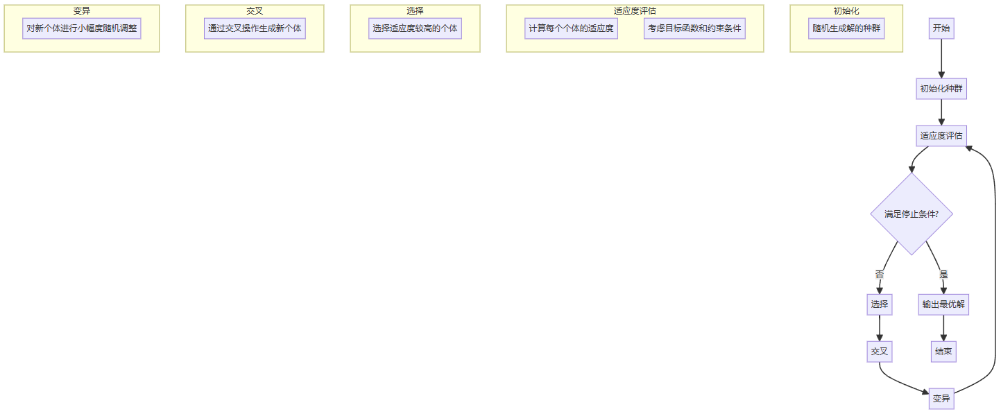
遗传算法
——此案例使用的代码是自定义实现的,追求方便简洁可以直接使用matlab的优化工具箱(GA)
步骤:
function nonlinear_ga()
    % 参数设置
    pop_size = 100;  % 种群大小
    max_iter = 500;  % 最大迭代次数
    crossover_rate = 0.8;  % 交叉概率
    mutation_rate = 0.2;  % 变异概率
    elite_size = 5;  % 精英个体数量
    bounds = [0, 5; 0, 3; 0, 3];  % 变量范围 [x1, x2, x3]

    % 初始化种群
    population = initialize_population(pop_size, bounds);

    % 遗传算法迭代
    for iter = 1:max_iter
        % 适应度评估
        fitness = evaluate_population(population);

        % 精英保留
        elites = elite_selection(population, fitness, elite_size);

        % 选择
        selected = tournament_selection(population, fitness);

        % 交叉
        offspring = crossover(selected, crossover_rate);

        % 变异
        mutated_offspring = mutation(offspring, mutation_rate, bounds);

        % 更新种群
        population = [elites; mutated_offspring];

        % 输出当前最优解
        [best_fitness, best_index] = min(evaluate_population(population));
        best_solution = population(best_index, :);
        fprintf('Iter: %d, Best Fitness: %.4f, Best Solution: [%s]\n', ...
            iter, best_fitness, num2str(best_solution));

        % 收敛检查
        if iter > 50 && std(fitness) < 1e-6
            fprintf('Algorithm converged.\n');
            break;
        end
    end

    % 最终结果
    [best_fitness, best_index] = min(evaluate_population(population));
    best_solution = population(best_index, :);
    fprintf('Final Best Fitness: %.4f, Best Solution: [%s]\n', ...
        best_fitness, num2str(best_solution));
end

function population = initialize_population(pop_size, bounds)
    population = zeros(pop_size, 3);
    for i = 1:pop_size
        population(i, :) = bounds(:, 1)' + (bounds(:, 2)' - bounds(:, 1)') .* rand(1, 3);
    end
end

function fitness = evaluate_population(population)
    fitness = zeros(size(population, 1), 1);
    for i = 1:size(population, 1)
        x1 = population(i, 1);
        x2 = population(i, 2);
        x3 = population(i, 3);

        % 目标函数
        obj_value = x1^2 + x2^2 + x3^2 + 8;

        % 约束条件
        g1 = x1^2 - x2 + x3^2;  % g1 >= 0
        g2 = 20 - (x1 + x2^2 + x3^3);  % g2 >= 0
        g3 = -x1 - x2^2 + 2;  % g3 = 0
        g4 = x2 + 2 * x3^2 - 3;  % g4 = 0

        % 惩罚项
        penalty = 0;
        penalty = penalty + max(0, -g1)^2;
        penalty = penalty + max(0, -g2)^2;
        penalty = penalty + abs(g3)^2;
        penalty = penalty + abs(g4)^2;

        % 适应度 = 目标值 + 惩罚项
        fitness(i) = obj_value + 1000 * penalty;
    end
end

function selected = tournament_selection(population, fitness)
    num_select = size(population, 1);
    selected = zeros(num_select, size(population, 2));
    for i = 1:num_select
        competitors = randi([1, num_select], 2, 1);
        if fitness(competitors(1)) < fitness(competitors(2))
            selected(i, :) = population(competitors(1), :);
        else
            selected(i, :) = population(competitors(2), :);
        end
    end
end

function elites = elite_selection(population, fitness, elite_size)
    [~, indices] = sort(fitness);
    elites = population(indices(1:elite_size), :);
end

function offspring = crossover(parents, crossover_rate)
    [num_parents, D] = size(parents);
    offspring = parents;

    for i = 1:2:num_parents-1
        if rand < crossover_rate
            crossover_point = randi([1, D-1]);
            offspring(i, :) = [parents(i, 1:crossover_point), parents(i+1, crossover_point+1:end)];
            offspring(i+1, :) = [parents(i+1, 1:crossover_point), parents(i, crossover_point+1:end)];
        end
    end
end

function mutated_offspring = mutation(offspring, mutation_rate, bounds)
    [num_offspring, D] = size(offspring);
    mutated_offspring = offspring;

    for i = 1:num_offspring
        for j = 1:D
            if rand < mutation_rate
                mutated_offspring(i, j) = bounds(j, 1) + (bounds(j, 2) - bounds(j, 1)) * rand;
            end
        end
    end
end
- 锦标赛选择方法: 锦标赛选择是一种常用的选择策略。在这种方法中,每次从种群中随机选择一小组个体(通常2-5个),然后从这一小组中选择适应度最高的个体。这种方法的优点是:
- 可以保持种群的多样性
- 选择压力可以通过调整锦标赛的规模来控制
- 计算效率较高,不需要对整个种群进行排序
- 精英保留策略: 精英保留确保每一代中最优秀的个体不会在进化过程中丢失。具体做法是:
- 在每一代中保留一定数量的最优个体
- 这些精英个体直接进入下一代,不经过交叉和变异操作
- 这种策略可以加快收敛速度,并保证算法的性能不会下降
- 惩罚函数法处理约束条件: 对于有约束的优化问题,惩罚函数法是一种将约束问题转化为无约束问题的方法。其原理是:
- 对违反约束的解施加惩罚,降低其适应度
- 惩罚的程度通常与违反约束的程度成正比
- 这种方法使得算法可以在搜索过程中探索可行解和不可行解的边界
- 收敛检查: 通过检查种群适应度的标准差来判断算法是否收敛是一种常用的终止条件。其原理是:
- 当种群中的个体趋于相似时,适应度的标准差会变小
- 设定一个阈值,当标准差小于这个阈值时,认为算法已经收敛
- 这种方法可以避免不必要的计算,在得到足够好的解时及时停止
案例背景:
\begin{equation}
f(\mathbf{x}) = 10n + \sum_{i=1}^{n} \left[ x_i^2 - 10\cos(2\pi x_i) \right]
\end{equation}
变量范围与极值
- 定义域:
xi∈[−5.12,5.12]∀i∈{1,2,…,n}xi∈[−5.12,5.12]∀i∈{1,2,…,n} - 全局最小值:
当 x=(0,0,…,0)x=(0,0,…,0) 时,f(x)=0f(x)=0。
%% 粒子群算法优化Rastrigin函数
clc; clear; close all;
%% 参数设置
n_particles = 50; % 粒子数量
n_dims = 2; % 问题维度
max_iter = 100; % 最大迭代次数
w = 0.729; % 惯性权重
c1 = 1.49445; % 个体学习因子
c2 = 1.49445; % 群体学习因子
pos_limit = [-5.12, 5.12]; % 位置范围
vel_limit = [-1, 1]; % 速度范围
%% 初始化粒子群
positions = rand(n_particles, n_dims) * (pos_limit(2)-pos_limit(1)) + pos_limit(1);
velocities = rand(n_particles, n_dims) * (vel_limit(2)-vel_limit(1)) + vel_limit(1);
fitness = rastrigin(positions);
p_best_pos = positions;
p_best_fit = fitness;
[g_best_fit, idx] = min(p_best_fit);
g_best_pos = p_best_pos(idx, :);
%% 主循环
best_fitness_history = zeros(max_iter, 1);
for iter = 1:max_iter
% 更新速度和位置
r1 = rand(n_particles, n_dims);
r2 = rand(n_particles, n_dims);
velocities = w*velocities + c1*r1.*(p_best_pos - positions) + c2*r2.*(g_best_pos - positions);
velocities = max(velocities, vel_limit(1));
velocities = min(velocities, vel_limit(2));
positions = positions + velocities;
positions = max(positions, pos_limit(1));
positions = min(positions, pos_limit(2));
% 计算新适应度
fitness = rastrigin(positions);
% 更新个体和群体最优
update_idx = fitness < p_best_fit;
p_best_pos(update_idx, :) = positions(update_idx, :);
p_best_fit(update_idx) = fitness(update_idx);
[current_best, idx] = min(p_best_fit);
if current_best < g_best_fit
g_best_fit = current_best;
g_best_pos = p_best_pos(idx, :);
end
best_fitness_history(iter) = g_best_fit;
end
%% 结果输出与可视化
fprintf('最优解位置: [%.4f, %.4f]\n', g_best_pos);
fprintf('最优适应度: %.4f\n', g_best_fit);
figure;
plot(best_fitness_history, 'LineWidth', 2);
xlabel('迭代次数');
ylabel('最优适应度');
title('收敛曲线');
grid on;
%% Rastrigin函数定义
function y = rastrigin(x)
y = 10 * size(x, 2) + sum(x.^2 - 10*cos(2*pi*x), 2);
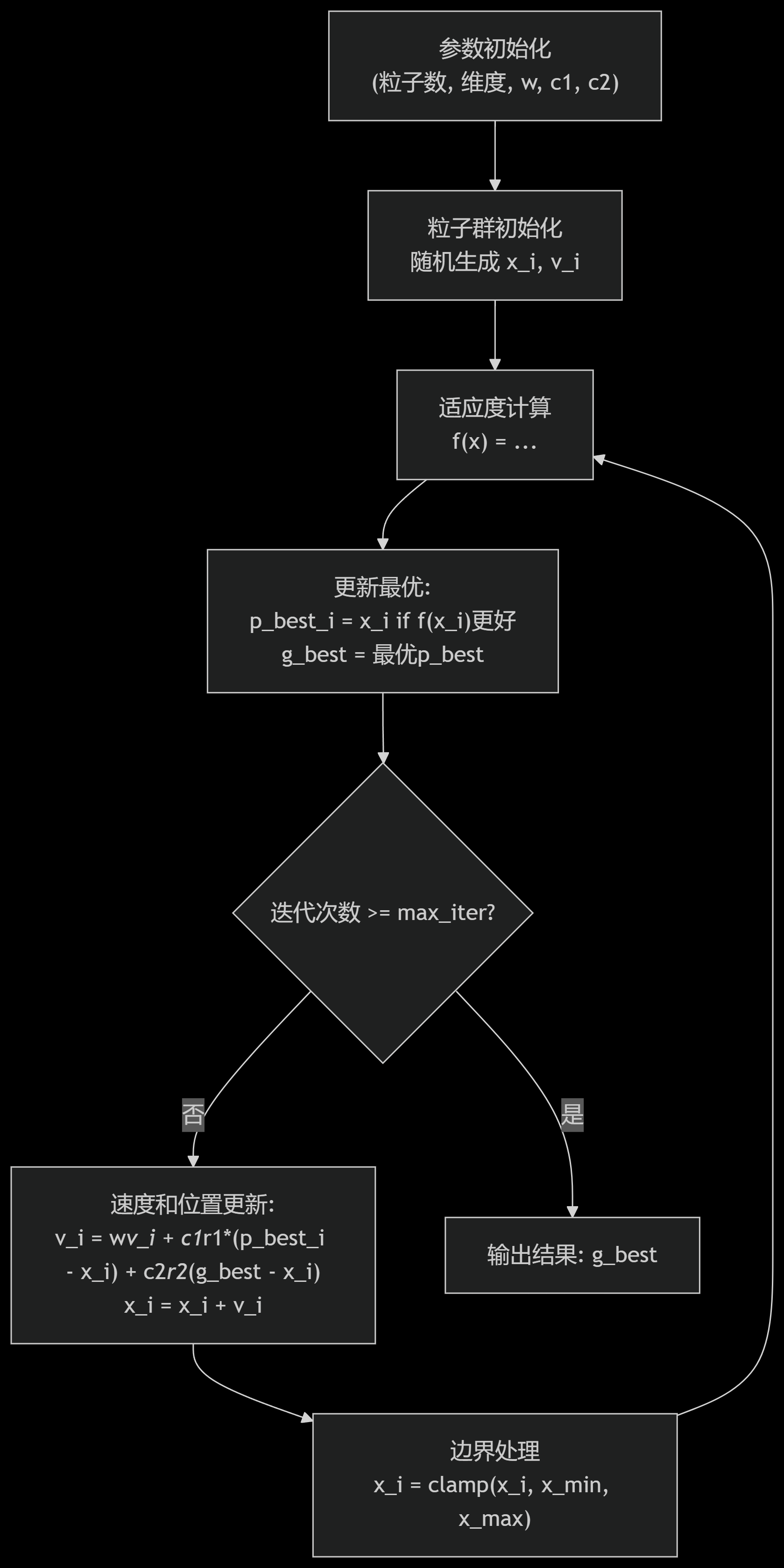
end代码解释
- 参数设置:选择50个粒子在2维空间搜索,惯性权重 ww 和学习因子 c1,c2c1,c2 的取值参考了经典PSO参数。
- 初始化:粒子的位置和速度在定义域内随机生成。
- 速度更新:根据个体历史最优和群体历史最优调整速度,速度被限制在 [−1,1][−1,1] 防止震荡。
- 边界处理:位置超出 [−5.12,5.12][−5.12,5.12] 时被截断到边界。
- 适应度计算:调用
rastrigin()函数计算每个粒子的目标函数值。 - 收敛曲线:记录每次迭代的全局最优值,直观展示算法收敛过程。
预测模型
案例:使用线性回归预测房屋价格
假设我们有一组房屋面积(平方米)与价格(万元)的数据,目标是建立线性模型,根据面积预测价格。
线性回归
——此案例使用的代码是自定义实现的,追求方便简洁可以直接使用matlab的优化工具箱(polyfit)
步骤:

% 生成模拟数据
rng(1);
area = 50 + 150 * rand(100, 1);
price = 50 + 0.8 * area + 10 * randn(100, 1);

% 数据分割
train_ratio = 0.8;
train_size = round(train_ratio * length(area));
train_indices = randperm(length(area), train_size);
test_indices = setdiff(1:length(area), train_indices);

X_train = area(train_indices);
y_train = price(train_indices);
X_test = area(test_indices);
y_test = price(test_indices);

% 数据归一化
[X_train_norm, mu, sigma] = zscore(X_train);
X_test_norm = (X_test - mu) / sigma;

% 特征扩展
X_train_ext = [ones(size(X_train_norm)), X_train_norm, X_train_norm.^2];
X_test_ext = [ones(size(X_test_norm)), X_test_norm, X_test_norm.^2];

% 定义损失函数(包含L2正则化)
lambda = 0.1;  % 正则化参数
computeCost = @(X, y, theta, lambda) (1/(2*length(y))) * sum((X * theta - y).^2) + (lambda/(2*length(y))) * sum(theta(2:end).^2);

% 梯度下降参数设置
theta = zeros(3, 1);
alpha = 0.1;
num_iters = 1000;
m = length(y_train);
J_history = zeros(num_iters, 1);

% 执行梯度下降(包含正则化)
for iter = 1:num_iters
    error = X_train_ext * theta - y_train;
    gradient = (1/m) * X_train_ext' * error + (lambda/m) * [0; theta(2:end)];
    theta = theta - alpha * gradient;
    J_history(iter) = computeCost(X_train_ext, y_train, theta, lambda);
end

% 模型评估
y_pred_train = X_train_ext * theta;
y_pred_test = X_test_ext * theta;
mse_train = mean((y_pred_train - y_train).^2);
mse_test = mean((y_pred_test - y_test).^2);
r2_train = 1 - sum((y_train - y_pred_train).^2) / sum((y_train - mean(y_train)).^2);
r2_test = 1 - sum((y_test - y_pred_test).^2) / sum((y_test - mean(y_test)).^2);

fprintf('训练集MSE: %.4f, R²: %.4f\n', mse_train, r2_train);
fprintf('测试集MSE: %.4f, R²: %.4f\n', mse_test, r2_test);

% 绘制结果
figure;
scatter(X_train, y_train, 'b', 'filled');
hold on;
scatter(X_test, y_test, 'r', 'filled');
X_range = linspace(min(area), max(area), 100)';
X_range_norm = (X_range - mu) / sigma;
X_range_ext = [ones(size(X_range_norm)), X_range_norm, X_range_norm.^2];
y_range = X_range_ext * theta;
plot(X_range, y_range, 'g-', 'LineWidth', 2);
xlabel('面积(平方米)');
ylabel('价格(万元)');
title('多项式回归拟合结果');
legend('训练数据', '测试数据', '回归线');
grid on;

% 预测新数据
new_area = 120;
new_area_norm = (new_area - mu) / sigma;
new_price = [1, new_area_norm, new_area_norm^2] * theta;
fprintf('面积为%d平方米的房屋预测价格为:%.2f万元\n', new_area, new_price);- 学习率自适应:可以实现自适应学习率,如Adam或RMSprop算法,以提高收敛速度和稳定性。
- 特征扩展:可以添加面积的平方项作为新特征,以捕捉非线性关系。
- 交叉验证:引入交叉验证来评估模型性能,避免过拟合。
- 正则化:添加L1或L2正则化项,以防止过拟合。
- 多元回归:考虑加入更多特征,如房间数量、地理位置等。
- 模型评估:计算并输出R²值、均方误差等指标来评估模型性能。
- 异常值处理:添加异常值检测和处理机制。
- 数据分割:将数据集分为训练集和测试集,以更好地评估模型泛化能力

Comments NOTHING